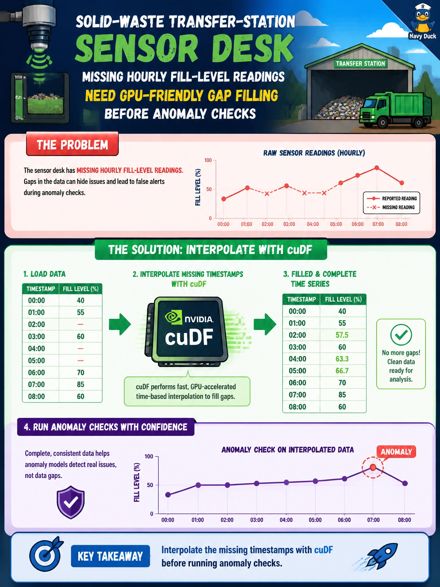
A solid-waste transfer-station sensor desk has missing hourly fill-level readings and wants GPU-friendly gap filling before anomaly checks. What should they use?

A solid-waste transfer-station sensor desk with missing hourly fill-level readings needs a continuous temporal grid before anomaly detection. Gaps break rolling statistics, lag features, and change-point logic that assume adjacent hours are comparable. The GPU-friendly associate practice is to interpolate missing timestamps with cuDF (or equivalent RAPIDS tooling) so the fill-level series is restored to an aligned hourly index at scale, then run anomaly checks on that reconstructed grid.

Deleting every hour with any missing sensor value across a whole month can erase large contiguous blocks and bias remaining data toward quieter periods, destroying the very patterns anomaly models should learn. Replacing gaps with a constant citywide average copied from last year’s annual report invents a flat, non-local signal that ignores station-specific dynamics and seasonal load. Leaving NaNs in place and training only on complete rows without aligning the clock yields irregular spacing; anomaly scores then mix true process shifts with sampling artifacts.

Exam caveat: interpolation is appropriate for short sensor dropouts when the physical process is continuous; it is not a license to invent values across known outages or multi-day failures without flags. cuDF accelerates the transform—it does not decide policy for which gaps may be filled.

Operational check: quantify missingness by hour and sensor, interpolate only within policy-approved gap lengths, retain a missingness indicator feature for the anomaly model, and spot-check filled windows against neighboring stations before promoting the pipeline.