
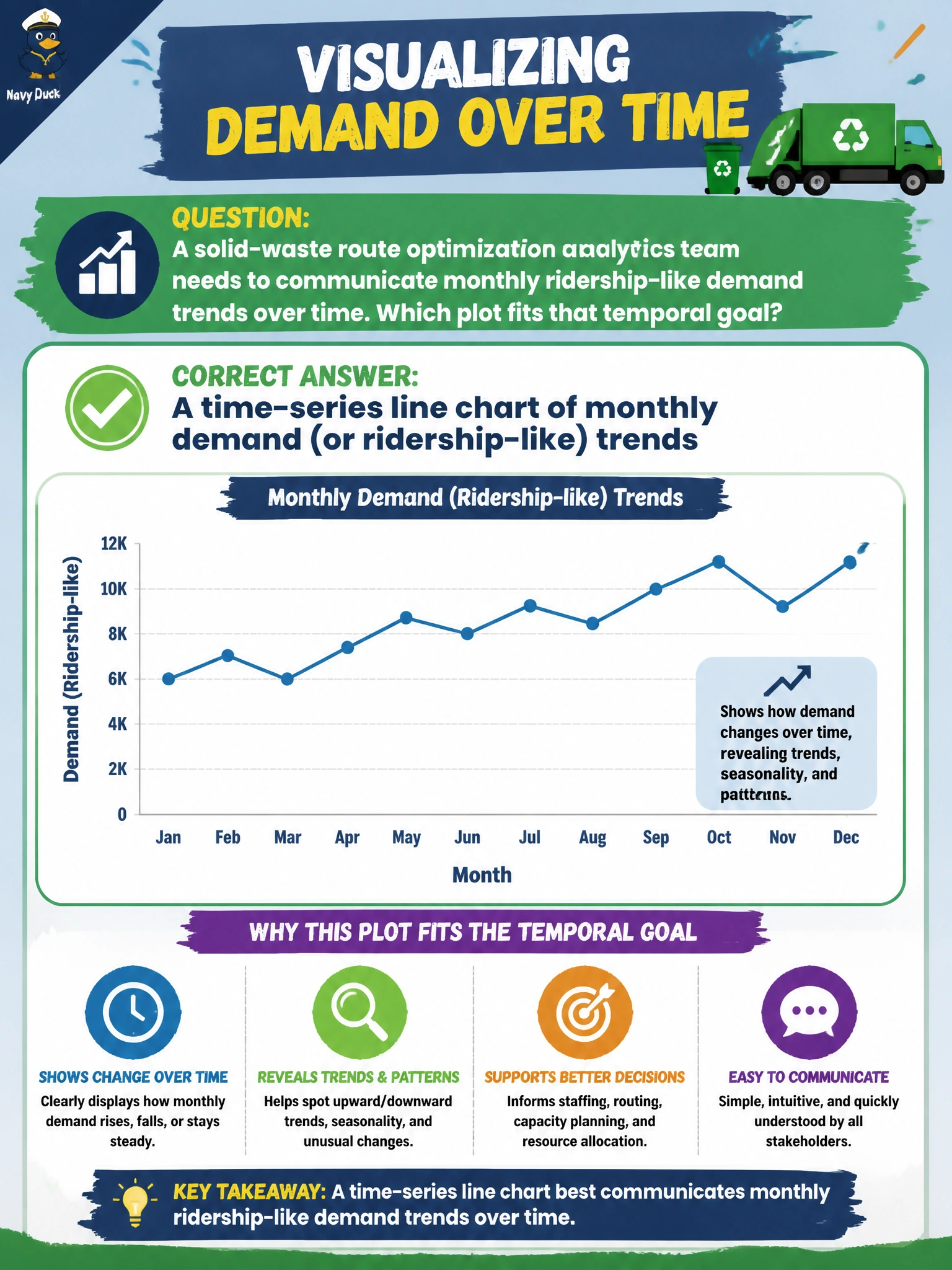
A solid-waste route optimization analytics team needs to communicate monthly ridership-like demand trends over time. Which plot fits that temporal goal?
Select an answer to reveal the explanation.
Short Explanation
You can follow monthly demand like a storyline with a time-series line chart, where rises and dips stay visible. A single-month pie, a choropleth that hides sequence, and a scatter without a temporal axis can’t show that trend.
Full Explanation
Communicating monthly demand (ridership-like) trends for solid-waste route optimization calls for a time-series line chart. By preserving chronological order, the line keeps rises, dips, seasonality, and level shifts visible—patterns route planners need when tonnage or stop demand changes month to month. Choose a plot to match the temporal goal, rather than using a chart that hides sequence. A pie chart of a single month has no time progression, so even correct slice proportions cannot show a monthly trend. A choropleth can show spatial intensity, but as described it hides the month-to-month sequence and does not meet the temporal goal. A scatter of unrelated vehicle IDs with no temporal axis shows neither demand over time nor a useful chronological pattern, so it distracts from the planning question. Exam caveat: a trend-over-time question calls for a time-series line chart; static pies and plots without a temporal axis do not communicate sequence. Practical check: aggregate demand by month using a consistent definition, label the axis units and starting month clearly, annotate known policy or holiday effects, and share the underlying monthly table with route planners for audit and reproducibility.