What is a practical benefit of using the RMSprop optimizer over plain SGD with a single fixed learning rate?
Select an answer to reveal the explanation.
Short Explanation and Infographic
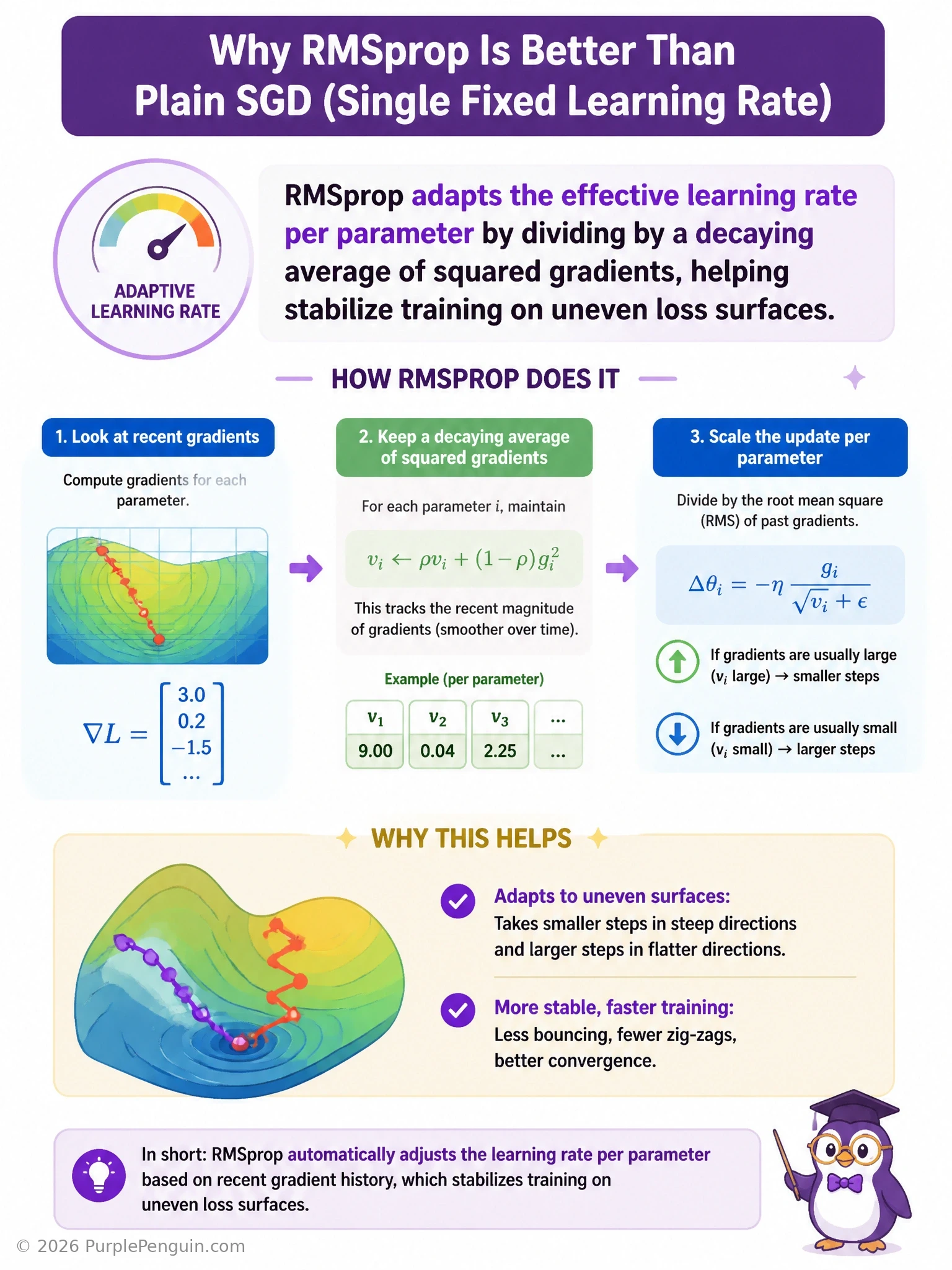
Plain SGD with one fixed learning rate treats every single parameter the same way, which is rough when your loss surface has steep cliffs in some directions and gentle slopes in others — one fixed step size just isn't right for all of them at once. RMSprop fixes that by dividing each parameter's update by a decaying average of that parameter's own squared gradients, so parameters getting big consistent gradients automatically get smaller effective steps, and parameters getting small gradients get relatively bigger steps. That's answer C, and it's a big reason RMSprop trains more smoothly on tricky, uneven loss landscapes — especially handy for recurrent networks. It doesn't guarantee zero oscillation, that's too strong a claim for any optimizer. It doesn't remove the need to pick an initial learning rate, you still set a base rate that RMSprop then adapts per parameter. And it has nothing to do with converting a classification problem into a regression one — that's determined by your loss function and output layer, not your optimizer.
Full explanation below image
Full Explanation
RMSprop improves upon plain SGD with a single fixed learning rate by maintaining a per-parameter, exponentially decaying moving average of squared gradients, and dividing the learning rate for each parameter by the square root of that average before applying the update. This means parameters associated with large, consistent gradients (steep directions in the loss surface) receive a smaller effective step size, while parameters with small or infrequent gradients (shallow directions) receive a relatively larger effective step. This per-parameter adaptivity helps training proceed more smoothly and stably on loss surfaces with very different curvature in different directions — a common challenge in deep and recurrent networks — compared to plain SGD, which applies the exact same learning rate uniformly to every parameter regardless of that parameter's gradient behavior.
The first distractor overstates what RMSprop can guarantee: while its adaptive scaling helps reduce oscillation caused by uneven gradient magnitudes across parameters, it does not make training immune to instability under all circumstances — an inappropriately chosen base learning rate or a pathological loss landscape can still cause problems. The second distractor is incorrect because RMSprop still requires an initial (base) learning rate hyperparameter to be specified; what it adapts is the effective per-parameter scaling applied on top of that base rate via the squared-gradient moving average, not the need to choose the base rate itself. The third distractor is incorrect because the choice between classification and regression is determined entirely by the task's output representation and corresponding loss function (for example, softmax with cross-entropy for classification versus a linear output with MSE for regression) — the optimizer used to minimize that loss (SGD, RMSprop, Adam, or otherwise) has no bearing on which type of task is being solved.
RMSprop was particularly influential for training recurrent neural networks, where gradients can vary dramatically in scale across time steps and parameters, making a single fixed learning rate poorly suited to the whole network. Its core mechanism — tracking a decaying average of squared gradients per parameter — was later combined with momentum (a decaying average of the raw gradients) in the Adam optimizer, which is now one of the most commonly used default optimizers across deep learning tasks.