
A customer with high late-afternoon use faces time-of-use rates with pricey 4-9 pm power, a monthly demand charge, and net metering that credits surplus at a lower rate. The seller must size self-use and export timing. Which rate-structure interpretation guides the preliminary estimate?
Select an answer to reveal the explanation.
Short Explanation
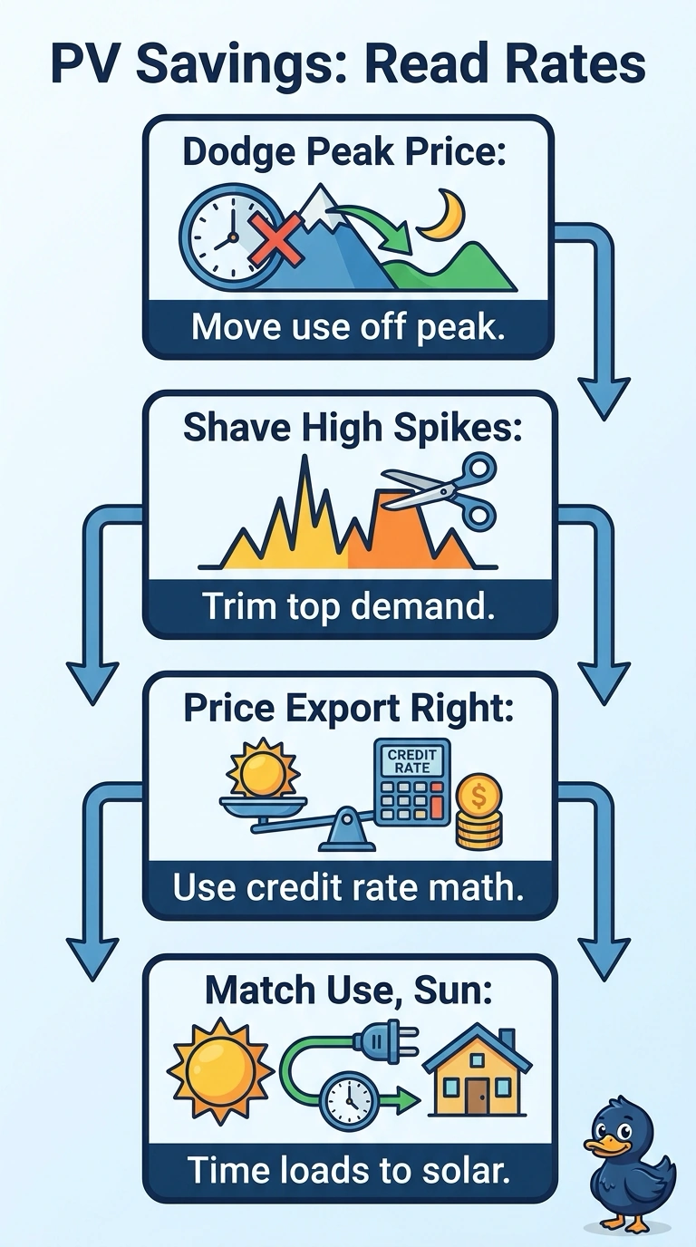
You’ll get a better preliminary estimate by shifting use out of the 4–9 p.m. peak, shaving demand spikes, and valuing exports at their lower credit rate. You’re accounting for both when power is used and how the tariff values it—that’s rate arbitrage.
Full Explanation
The correct interpretation reflects all three cost signals: shift flexible consumption away from the costly 4–9 p.m. period, reduce monthly peak demand because it drives a separate demand charge, and value exported energy at the lower net-metering credit rather than the retail purchase rate. Shifting loads out of peak and shaving demand spikes are sound, but valuing exports at retail assumes a more favorable compensation rule than the stated lower credit, overstating surplus-generation value. Shifting loads out of peak and valuing exports at the lower credit correctly account for timing and export compensation, but tracking energy charges alone omits the monthly demand charge and can miss savings from reducing the billing-period maximum. Shaving demand spikes and using the lower credit are appropriate, but shifting loads out of a midday peak targets the wrong period; it may leave costly 4–9 p.m. use unchanged. Exam caveat: a demand charge may depend on a short interval’s maximum kW, not total monthly kWh, and tariff details can specify measurement periods or seasons. As a practical check before sizing, review interval-load data alongside the applicable tariff, confirm the demand-charge interval and export-credit schedule, and estimate self-consumption and exports by time of day.