
A home-internet provider regresses monthly bill on plan type, then adds a predictor that leaves every fitted bill unchanged, so plain R-squared stays the same and short of a perfect fit. What happens to adjusted R-squared?
Select an answer to reveal the explanation.
Short Explanation
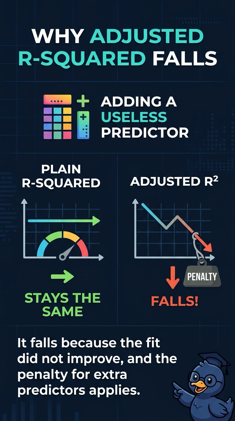
Plain R-squared stays where it is when you add a predictor that does not change the fitted values. Adjusted R-squared charges rent for the extra column, so the same fit spread over more columns makes it fall. The trap is assuming the two scores have to move together.
Full Explanation
Plain R-squared is the share of bill variation captured by the fitted values. Adding a predictor cannot reduce that share in an ordinary linear fit, and in this case the fitted bills do not change, so plain R-squared stays exactly where it was. Adjusted R-squared reduces that score to charge for the number of predictors. With the unexplained share unchanged and still above zero, because the fit is short of perfect, the heavier penalty for one more predictor pulls adjusted R-squared down. It does not rise in lockstep with plain R-squared; the plain score did not rise, and the adjusted score is not a rescaling that preserves every move. It also does not stay equal to plain R-squared, because the penalty term changes as soon as the predictor count changes, even though the fitted values did not. The adjustment is defined for a numeric outcome such as a bill and is not limited to categorical predictors, so it does not become undefined here. Exam caveat: if a new predictor improves the fit enough to outweigh the penalty, adjusted R-squared can rise; that is a different case from an unchanged fit. Operational check: recompute adjusted R-squared from the unchanged plain R-squared, the sample size, and the new predictor count, and confirm the adjusted value is lower.