
Compared with plain stochastic gradient descent (SGD), what is the primary benefit of using RMSProp as an optimizer?
Select an answer to reveal the explanation.
Short Explanation and Infographic
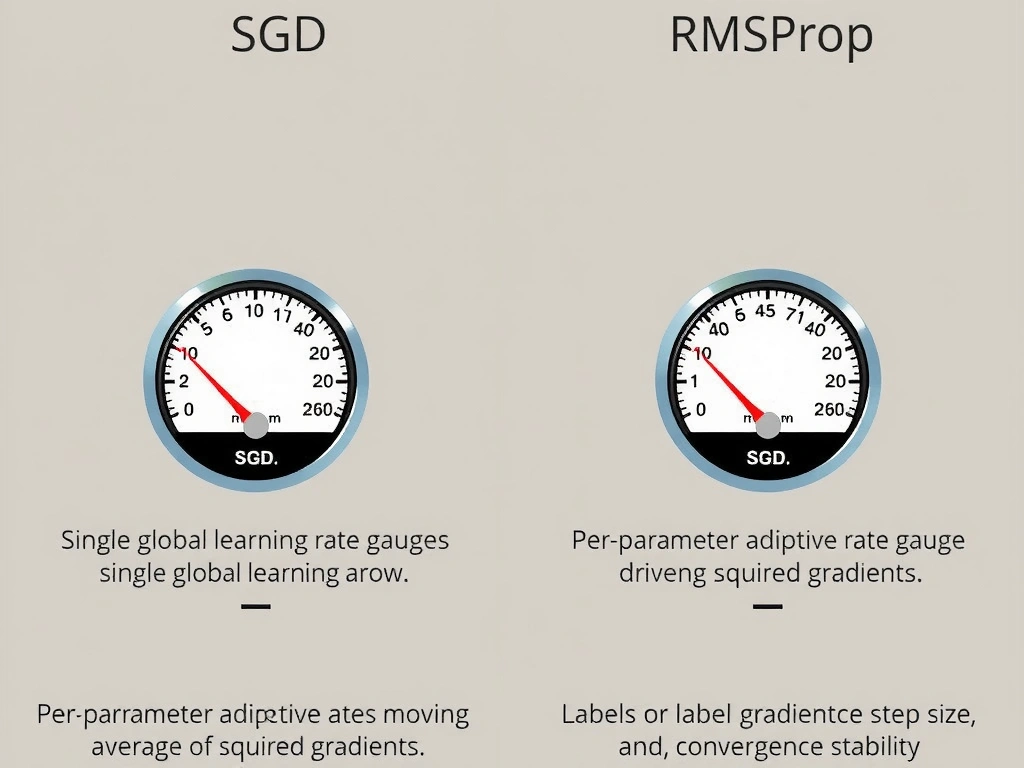
Here's the deal with optimizers: plain SGD takes the same-size step (more or less) for every weight, and that can get ugly when some gradients are huge and others are tiny. RMSProp fixes a lot of that headache. Think of it like cruise control that reacts per lane—each parameter gets its own effective learning rate based on a running average of recent squared gradients. Big, noisy dimensions get damped; quiet ones can still move. Boss walks in asking why training stalled on sparse features? Adaptive methods like RMSProp are often the answer. Trap: people confuse “adaptive” with “solves vanishing gradients forever”—nope. Takeaway: RMSProp beats vanilla SGD mainly by adapting step sizes per parameter so training converges more smoothly.
Full explanation below image
Full Explanation
Stochastic gradient descent updates parameters using the gradient of the loss with respect to a mini-batch, typically with one global learning rate. That simplicity is powerful but brittle: coordinates with large gradient magnitudes can overshoot, while coordinates with small gradients crawl, especially when features or layers have very different scales. RMSProp (Root Mean Square Propagation) addresses this by maintaining an exponentially weighted moving average of squared gradients for each parameter. The update divides the current gradient by the square root of that average (plus a small epsilon for numerical stability), producing an effectively adaptive learning rate per weight.
This per-parameter adaptation is the main practical advantage over plain SGD. In regions where gradients have been large for some time, RMSProp shrinks steps; where gradients have been small, steps remain relatively larger. That often yields faster and more stable convergence on non-convex deep learning objectives without requiring as much manual learning-rate babysitting. Related adaptive methods (AdaGrad, Adam) share the same spirit—history-aware scaling—but the exam-relevant contrast with SGD is adaptivity versus a single fixed rate.
The distractors capture common misconceptions. RMSProp is not vision-only; it appears across NLP, tabular, and multimodal training. It does not “solve” vanishing gradients the way gating architectures (LSTM/GRU) or residual connections do—those change how signal flows through depth or time. Claiming RMSProp uses a constant rate while SGD uses a variable one flips the truth: baseline SGD is the constant-rate method (unless an external schedule is added), and RMSProp’s defining feature is adaptive scaling.
In practice, teams still tune a base learning rate, decay schedules, and batch size even with adaptive optimizers. Memory of past squared gradients can also interact with non-stationary objectives, so monitoring loss curves remains essential. For certification and production intuition alike: when asked what RMSProp buys you over SGD, answer adaptive per-parameter learning rates that improve stability and often speed convergence—not modality specialization or magic fixes for architectural gradient pathologies.